
Function Approximation and Ordinary Least Squares
200 years of Statistical Machine Learning

The mathematics of least squares would have been so trivial for Gauss that even had he come upon the method he might have passed it over as but one of many, not noticing its true significance until Legendre’s book prodded his memory and produced a post facto priority claim.

There have been many extraordinary equations that changed the world (whether they were discovered or invented depends on whether you subscribe to mathematical Platonism—I do) but among the 17 equations that changed the world, the legendary Ordinary Least Squares (OLS) wasn’t listed among them (though it is heavily related to both the Normal Distribution and Information Theory).
It’s a shame because the article and tweets referencing the “17 Equations” have been floating around for nearly ten years.
So I will tell you about the magic of OLS, a little about its history, some of its extensions, and its applications (yes, to Fintech too).
Gauss and the Invention of Least Squares
One of my favorite authors and historical statisticians Dr. Stephen Stigler published a wonderful historical review in 1981 titled Gauss and the Invention of Least Squares. He argued that the prolific Carl Freidrich Gauss discovered OLS in 1809 and fundamentally shaped the future of science, business, and society as we know it.
But first, what is OLS and why is it important?
OLS is often referred to by many things across several different disciplines, some of them are:
Linear Regression
Multivariate Regression
The Normal Equations
Maximum Likelihood
Method of Moments
Singular Value Decomposition of Xw−y=U(Σ′w−U′−y)Xw−y=U(Σ′w−U′−y)
But all of them ultimately reflect the same mathematical expression and the same solution to the sum of squares of the regression equation (in scalar notation).
A little mathematics yields the famous OLS estimator (i.e., equation)
Or in matrix notation:
This equation is pure sorcery.
From it humans have been gifted the knowledge and ability to make inference about drug treatments, forecast the weather, predict genes, make empirically grounded recommendations about public health, understand the galaxies, and, yes, even develop artificially intelligent chatbots.
But it all started with OLS.
The equation basically says "Look at data about x and estimate a linear relationship with y by minimizing the average error."
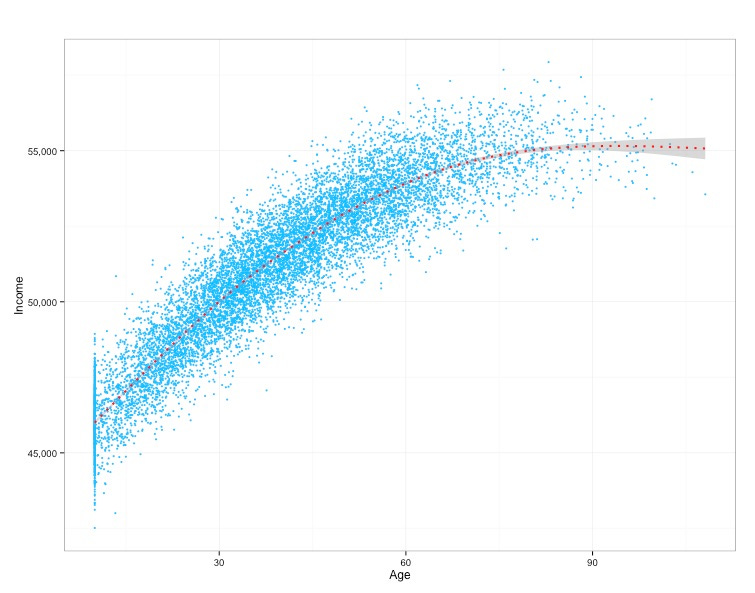
As a concrete example, suppose you wanted to know the relationship between Age and Income (a simplification of the well-studied Mincer Equation, how would you figure this out? A simple linear regression could estimate that relationship and the β1 would represent the partial-correlation (sometimes called the marginal effect2 or coefficient estimate) and it exactly represents the slope of the line below.

Isn't that just amazing?
To think Gauss had discovered OLS as a method of calculating the orbits of celestial bodies (i.e., he discovered regression as a sub-problem) and that today, over 200 years later, humans would use it to for so much of what we do is astounding.
Over the years statisticians, economists, computer scientists, engineers, psychometricians, and other researchers have advanced OLS in such profound and unique ways. Some of them have been used to reflect data generated from more non-standard distributions (e.g., a Weibull distribution), or to frame analytical problems to use prior information in a structured way (e.g., through Bayesian Inference), while others have enhanced these equations to learn high-dimensional nonlinear functions (e.g., via Neural Networks or Gradient Boosting). All of which are extensions of Gauss’ extraordinary work.
Function Approximation
I showed above that regression (OLS) can be used to fit a line through two variables (e.g., Age and Income), which basically assumes you want to estimate a linear relationship…but wait there’s more!
As I said, the statistics and machine learning community did a lot of great work over the last 200+ years and now we can model more sophisticated relationships.
Let’s go back to our example of Age and Income.
In the graph above we saw that the relationship fit the data quite linearly (by the way this is by construction because I simulated the data)…but what if it wasn't linear?
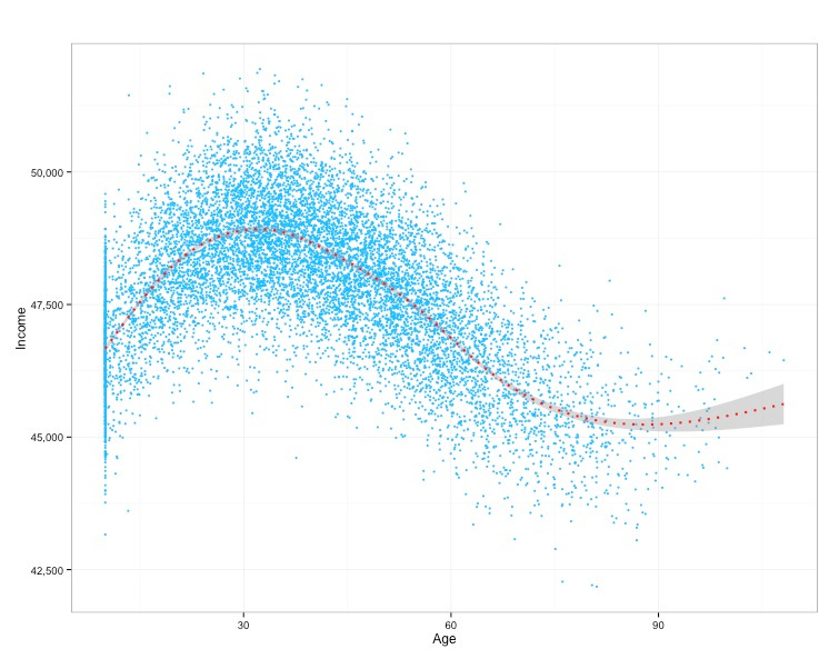
What if we knew Age only increased Income to a degree and that the marginal return was decreasing? Well, maybe we'd see a plot like below.
What if things were a little less intuitive and, after another point, your Income (on average) started to go back up again? We could see something like this:
Or what if we saw something that was just, well, plain weird?
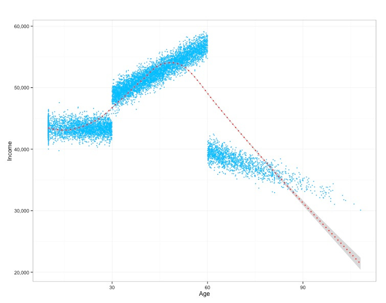
The graph above is my favorite example because it shows a piecewise linear function and, while strange looking, relationships like these are very common phenomena in the wild. That is to say that in real life (particularly with humans) correlation between things is rarely continuous, smooth, and fully linear. It’s typically discontinuous at weird points, sometimes inflated at a random point, and not as easy on the eyes.
This is because we are usually modeling behaviors, decisions, or processes by human generated systems in the world, and those systems often have weird boundary points/thresholds that dictate or mean something. In fact, I wrote about this before where I said rather explicitly that Financial data is Chaos.
Now going back to the example of Age and Income, weird trends in the data arise in the US because states have certain age minimums, some people decide to seek post-secondary education without working, some people are physically unable to work, and a bunch of other unknown things that mean something…so you see partial correlations that aren’t so clean as my simulation above or that they show you in graphs in textbooks.
Scatter plots lack nuance because they are by definition two dimensional and are only meant to elucidate a crude understanding of two things coexisting in the world. Simple things are often truisims at the aggregate level but rarely true at the individual level.
While the correlation in this example isn’t strictly linear, if you account for the nonlinear nature of it you actually end up with a fairly strong correlation.
Simpson’s Paradox, Interactions, and the Curse of Dimensionality
So we know that correlation can exist between things and that it can be both nonlinear and strong, but sometimes there’s more to the data. Often we’re only able to scratch the surface on what’s available. This is well understood in the statistical/econometric literature and is referred to as Omitted Variable Bias or Simpson’s Paradox.

In summary, when looking at data, you can always be missing one piece of information that could flip your conclusions. While that is always theoretically possible, sometimes this isn’t that likely but that doesn’t change it from being a possibility.
Said another way, what looks true in one dimension may not be true in more dimensions and the reverse.
In general, as you increase the dimensionality (i.e., the number of attributes you’re looking at for some set of data) there’s just a lot more uncertainty. Unfortunately, our brains can’t really comprehend high dimensions too well but computers absolutely can and that’s really where the fun starts.
The additional challenge here is that often, though not always, we’re faced with more information than data points. More attributes than samples or more variables than records. In Statistics, this is called the Curse of Dimensionality.
For OLS in particular, it means we can’t actually compute the OLS estimator because the underlying matrix is not invertible and, in general, the amount of data required to get robust function approximations grows exponentially with the dimensionality. In a way, more dimensions/attributes means you have to make inferences in higher dimensional spaces with less confidence.
But if you throw out your regard for the coefficients/weights (i.e., the solution to the OLS equation) explicitly and treat the whole thing as an optimization problem, you can predict something very well. This is the power of Gradient Boosting and Neural Networks.
Gradient Boosting and Neural Networks are two broad classes of algorithms that are powerful tools in learning high-dimensional, nonlinear functions.
Let’s see this with two examples.
How Computers Recognize Digits

In the picture above we have a two dimensional drawing (which I did) of the integer “2” being run through a simple Convolutional Neural Network.
Note: It’s two dimensions because there is a length and width. Most modern images are 3-dimensional because there is an explicit dimension for color (known as the RGB coordinate) but there is no color here (only grayscale) so we don’t need the RGB dimension.
The network that decided my drawing of a “2” was actually a “2” learned a nonlinear function and interactions of the pixels/data-points through the core operations of neural networks: matrix multiplications, hidden layers, activation functions, the convolution operation, stochastic gradient descent, and backpropagation.

In less jargony words, the network reads chunks of the image, makes some initial guesses about what the function is, does some multiplications and summations to try to predict what number it is, and updates the network based on how good it did at guessing.
These core ingredients are the magic that make Deep Learning so powerful. The mathematics behind it is surprisingly simple and that’s kind of what makes it so wonderful: intelligence is rooted in elegant simplicity.
To make this a little more concrete with a numerical example, the gif below shows the behavior of the convolution operation with 2 filters (weights) being applied to an image with color. Notice that the convolution is applying the red filters (W0 and W1) and bias (b0 and b1) to each RGB dimension (the 3 large left gray grids called Input Volume), which results in the 2 green grids called “Output Volume”.
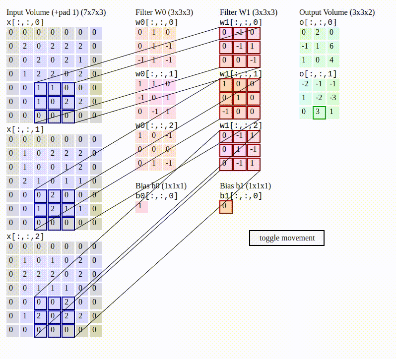
This is how local correlation of pixels is exploited in the convolution operation— by sliding through the image and applying the filters. This movement helps the network measure data in images near each other and build some meaningful representation from it, similar to how humans use our eyes and visual cortex to see where a cliff ends so we don’t walk off of it.
Things can get much more sophisticated from here in Deep Learning but I won’t discuss that as I’d need to write a book to scratch the surface. I do recommend reading the Deep Learning Book for those interested.
How Computers Mine Data
I wrote before about how Neural Networks, while fantastic across many problem spaces, have not been nearly as effective on tabular data as Gradient Boosted Trees. In summary, it’s because tabular data is rather discrete in nature and typically constructed by arbitrary boundaries and Gradient Boosting Machines (GBMs) joyfully exploit this property of the data.
The underlying algorithm powering Gradient Boosted Decision Trees has 4 core ingredients:
Greedily sorting the data and taking local averages
Recursively partitioning the data across dimensions
Sequentially updating the predictions by using the residual in each new iteration
Aggregating across hundreds (or thousands) of weak models
Restating this again with less jargon (and being a little reductionist), GBMs are basically really, really intense decision trees. There are some important implementation details to make it so powerful but the essence of it really can be reduced to fancy sorting.
And this fancy sorting works wonders.
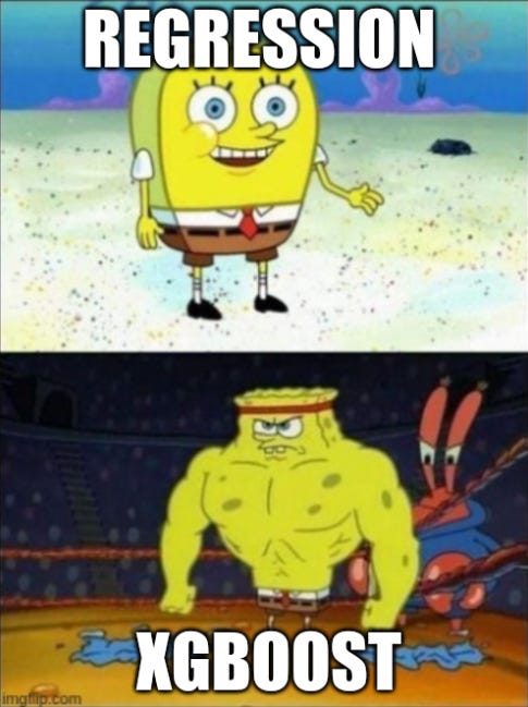
Outside of Deep Learning, XGBoost really has been the algorithm of choice when building in ML (at least in the private sector and data mining competitions) and it’s because it is just so effective.

As an example, I simulated a trivial discontinuous nonlinear two dimensional function (shown above) and trained a Neural Network and a GBM to learn it. You’ll see that XGBoost learns this function extremely quickly (after about 6 iterations) while the NN spends a lot of time oscillating back and forth.
Note: I’m sure I could tune the NN to learn this but I used both algorithms out of the box and I actually had to tune the GBM step size down to slow how quickly it learns the function. The point is how easily GBMs work out of the box.
The examples above show how GBMs and NNs can trivially learn nonlinear functions and the exciting thing is that this generalizes to higher dimensions too. For Neural Networks they can learn amazing (often smooth) structures or rich high dimensional embeddings while GBMs quickly learn complex discrete surfaces.
And the applications, as I said before, are everywhere.
Fintech and the Anarchy of Rules
If you’ve worked in Fintech, you’ll know that Rules/Decision engines are ubiquitous. During my time at Goldman we had 3 (just for one business vertical 🥲).
These systems are typically used to define rules applied to some piece(s) of data that usually map to some outcome. For example, “If Credit Score >= 630, Approve the customer for a loan”.
Inevitably, risk teams start to add lots of stuff here and what starts out as a simple set of rules becomes tens of thousands of lines of complexity. Engineers know that this is the natural evolution of any service but those not familiar with software engineering best practices may be surprised at how hard it becomes to make changes to these systems, and the inevitable cost is the speed of execution.
This spiral into chaos and anarchy happens little by little as one business analyst after the next finds a segment that can improve some metric by some percentage, and another analyst finds another subsegment, and so on…until you have a monstrosity of rules that impact your latency and your understanding of what’s actually happening in your business.
More importantly, what you have actually done is built a large decision tree—with maybe more (or less!) human intelligence reflected in some areas—which is basically to say that you’ve used several humans to define a decision boundary over multiple dimensions.
Is that optimal?
Maybe! There are a lot of regulatory constraints within Fintech that make humans defining the logic and math of these systems fairly pragmatic.
But, as we saw before, what can be true in one dimension may not be true in several dimensions, so I recommend you be extremely data driven in your meta analysis—i.e., the analysis of your analysis. This will help you learn, adapt, and iterate much faster. More importantly, it will help you balance pragmatism and good statistical machine learning practices.
To be explicit, make sure you actually go back and quantify whether the rules you’ve constructed actually ended up being statistically significant and useful, or if they were just guessing. Guessing is dumb and it will ruin your business, and we don’t want that so make sure to bust out the big guns (i.e., XGBoost). You will thank me when your vintages mature.
Conclusion
We humans try to make predictions, inferences, and guesses about the world. Often based on limited data.
This is both good and natural but we have to keep in mind that we look at data and the world through few dimensions, with imperfect information, and with—probably—a biased sample.
So exercise a healthy amount of self-skepticism and ask yourself what information you could be missing that could flip your conclusion or whether you’re just looking at a narrow segment of data where your conclusions won’t extrapolate. Over the long term, you will make better decisions and better predictions.
Happy function approximating!
-Francisco
Some Content Recommendations
Jason Mikula and Fintech Takes held another wonderful podcast this time covering the dismantling of Goldman’s Marcus, among other things. As always, the dynamic duo have a really great discussion. This time covering Gen Z Banking, Crypto Crashes, and some 2023 predictions. These are two of my absolute favorite writers in Fintech so getting to listen to them on a podcast is real joy.
JareaufromBatch Processingwrote a fantastic article on Payment Companies and Profitability and how Adyen is crushing it.
Simon Taylor fromFintech Brain Food 🧠 authored another brilliant piece, this time covering The Fintech Hype Cycle. Some of my favorite parts of this were his thoughts on Generative AI (which I 100% agree with), his take on POS Payments, and his analysis of Goldman’s lending losses (which contextualizes the $1.2 billion in losses with revenue because that is the only thing that actually matters in lending).
Alex Xu fromByteByteGo Newsletter, the best newsletter for software engineering content, wrote about Designing a Chat Application, CI/CD pipelines, Visa Disputes and Chargebacks, and how to deploy services to production. It was great as always.
Postscript
Did you like this post? Do you have any feedback? Do you have some topics you’d like me to write about? Do you have any ideas how I could make this better? I’d love your feedback!
Feel free to respond to this email or reach out to me on Twitter! 🤠
There should be a hat on this but Substack does not yet support in-line LaTeX rendering, but I appreciate that Substack recently launched LaTeX rendering at all!
We all know that marginal effect should not be mistaken for causality. 😉